Note
Click here to download the full example code
Modeling with interval averages
Transposing interval-averaged irradiance data
This example shows how failing to account for the difference between instantaneous and interval-averaged time series data can introduce error in the modeling process. An instantaneous time series represents discrete measurements taken at each timestamp, while an interval-averaged time series represents the average value across each data interval. For example, the value of an interval-averaged hourly time series at 11:00 represents the average value between 11:00 (inclusive) and 12:00 (exclusive), assuming the series is left-labeled. For a right-labeled time series it would be the average value between 10:00 (exclusive) and 11:00 (inclusive). Sometimes timestamps are center-labeled, in which case it would be the average value between 10:30 and 11:30. Interval-averaged time series are common in field data, where the datalogger averages high-frequency measurements into low-frequency averages for archiving purposes.
It is important to account for this difference when using interval-averaged weather data for modeling. This example focuses on calculating solar position appropriately for irradiance transposition, but this concept is relevant for other steps in the modeling process as well.
This example calculates a POA irradiance timeseries at 1-second resolution as a “ground truth” value. Then it performs the transposition again at lower resolution using interval-averaged irradiance components, once using a half-interval shift and once just using the unmodified timestamps. The difference affects the solar position calculation: for example, assuming we have average irradiance for the interval 11:00 to 12:00, and it came from a left-labeled time series, naively using the unmodified timestamp will calculate solar position for 11:00, meaning the calculated solar position is used to represent times as far as an hour away. A better option would be to calculate the solar position at 11:30 to reduce the maximum timing error to only half an hour.
import pvlib
import pandas as pd
import matplotlib.pyplot as plt
First, we’ll define a helper function that we can re-use several times in the following code:
def transpose(irradiance, timeshift):
    """
    Transpose irradiance components to plane-of-array, incorporating
    a timeshift in the solar position calculation.

    Parameters
    ----------
        irradiance: DataFrame
            Has columns dni, ghi, dhi
        timeshift: float
            Number of minutes to shift for solar position calculation
    Outputs:
        Series of POA irradiance
    """
    idx = irradiance.index
    # calculate solar position for shifted timestamps:
    idx = idx + pd.Timedelta(timeshift, unit='min')
    solpos = location.get_solarposition(idx)
    # but still report the values with the original timestamps:
    solpos.index = irradiance.index

    poa_components = pvlib.irradiance.get_total_irradiance(
        surface_tilt=20,
        surface_azimuth=180,
        solar_zenith=solpos['apparent_zenith'],
        solar_azimuth=solpos['azimuth'],
        dni=irradiance['dni'],
        ghi=irradiance['ghi'],
        dhi=irradiance['dhi'],
        model='isotropic',
    )
    return poa_components['poa_global']
Now, calculate the “ground truth” irradiance data. We’ll simulate clear-sky irradiance components at 1-second intervals and calculate the corresponding POA irradiance. At such a short timescale, the difference between instantaneous and interval-averaged irradiance is negligible.
# baseline: all calculations done at 1-second scale
location = pvlib.location.Location(40, -80, tz='Etc/GMT+5')
times = pd.date_range('2019-06-01 05:00', '2019-06-01 19:00',
                      freq='1s', tz='Etc/GMT+5')
solpos = location.get_solarposition(times)
clearsky = location.get_clearsky(times, solar_position=solpos)
poa_1s = transpose(clearsky, timeshift=0)  # no shift needed for 1s data
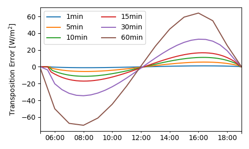
Now, we will aggregate the 1-second values into interval averages. To see how the averaging interval affects results, we’ll loop over a few common data intervals and accumulate the results.
fig, ax = plt.subplots(figsize=(5, 3))

results = []

for timescale_minutes in [1, 5, 10, 15, 30, 60]:

    timescale_str = f'{timescale_minutes}min'
    # get the "true" interval average of poa as the baseline for comparison
    poa_avg = poa_1s.resample(timescale_str).mean()
    # get interval averages of irradiance components to use for transposition
    clearsky_avg = clearsky.resample(timescale_str).mean()

    # low-res interval averages of 1-second data, with NO shift
    poa_avg_noshift = transpose(clearsky_avg, timeshift=0)

    # low-res interval averages of 1-second data, with half-interval shift
    poa_avg_halfshift = transpose(clearsky_avg, timeshift=timescale_minutes/2)

    df = pd.DataFrame({
        'ground truth': poa_avg,
        'modeled, half shift': poa_avg_halfshift,
        'modeled, no shift': poa_avg_noshift,
    })
    error = df.subtract(df['ground truth'], axis=0)
    # add another trace to the error plot
    error['modeled, no shift'].plot(ax=ax, label=timescale_str)
    # calculate error statistics and save for later
    stats = error.abs().mean()  # average absolute error across daylight hours
    stats['timescale_minutes'] = timescale_minutes
    results.append(stats)

ax.legend(ncol=2)
ax.set_ylabel('Transposition Error [W/m$^2$]')
fig.tight_layout()

df_results = pd.DataFrame(results).set_index('timescale_minutes')
print(df_results)
Out:
                   ground truth  modeled, half shift  modeled, no shift
timescale_minutes
1.0                         0.0             0.012018           0.702429
5.0                         0.0             0.021197           3.542882
10.0                        0.0             0.062650           7.051620
15.0                        0.0             0.142984          10.531453
30.0                        0.0             0.581701          20.619625
60.0                        0.0             1.955845          39.418585
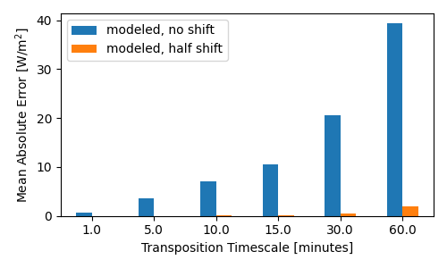
The errors shown above are the average absolute difference in \(W/m^2\). In this example, using the timestamps unadjusted creates an error that increases with increasing interval length, up to a ~40% error at hourly resolution. In contrast, incorporating a half-interval shift so that solar position is calculated in the middle of the interval instead of the edge reduces the error by one or two orders of magnitude:
fig, ax = plt.subplots(figsize=(5, 3))
df_results[['modeled, no shift', 'modeled, half shift']].plot.bar(rot=0, ax=ax)
ax.set_ylabel('Mean Absolute Error [W/m$^2$]')
ax.set_xlabel('Transposition Timescale [minutes]')
fig.tight_layout()
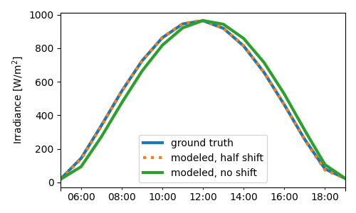
We can also plot the underlying time series results of the last iteration (hourly in this case). The modeled irradiance using no shift is effectively time-lagged compared with ground truth. In contrast, the half-shift model is nearly identical to the ground truth irradiance.
fig, ax = plt.subplots(figsize=(5, 3))
ax = df.plot(ax=ax, style=[None, ':', None], lw=3)
ax.set_ylabel('Irradiance [W/m$^2$]')
fig.tight_layout()
Total running time of the script: ( 0 minutes 2.017 seconds)