Note
Click here to download the full example code
Backtracking on sloped terrain
Modeling backtracking for single-axis tracker arrays on sloped terrain.
Tracker systems use backtracking to avoid row-to-row shading when the
sun is low in the sky. The backtracking strategy orients the modules exactly
on the boundary between shaded and unshaded so that the modules are oriented
as much towards the sun as possible while still remaining unshaded.
Unlike the true-tracking calculation (which only depends on solar position),
calculating the backtracking angle requires knowledge of the relative spacing
of adjacent tracker rows. This example shows how the backtracking angle
changes based on a vertical offset between rows caused by sloped terrain.
It uses pvlib.tracking.calc_axis_tilt() and
pvlib.tracking.calc_cross_axis_tilt() to calculate the necessary
array geometry parameters and pvlib.tracking.singleaxis() to
calculate the backtracking angles.
Angle conventions
First let’s go over the sign conventions used for angles. In contrast to fixed-tilt arrays where the azimuth is that of the normal to the panels, the convention for the azimuth of a single-axis tracker is along the tracker axis. Note that the axis azimuth is a property of the array and is distinct from the azimuth of the panel orientation, which changes based on tracker rotation angle. Because the tracker axis points in two directions, there are two choices for the axis azimuth angle, and by convention (at least in the northern hemisphere), the more southward angle is chosen:
Note that, as with fixed-tilt arrays, the axis azimuth is determined as the angle clockwise from north. The azimuth of the terrain’s slope is also determined as an angle clockwise from north, pointing in the direction of falling slope. So for example, a hillside that slopes down to the east has an azimuth of 90 degrees.
Using the axis azimuth convention above, the sign convention for tracker rotations is given by the right-hand rule. Point the right hand thumb along the axis in the direction of the axis azimuth and the fingers curl in the direction of positive rotation angle:
So for an array with axis_azimuth=180 (tracker axis aligned perfectly
north-south), pointing the right-hand thumb along the axis azimuth has the
fingers curling towards the west, meaning rotations towards the west are
positive and rotations towards the east are negative.
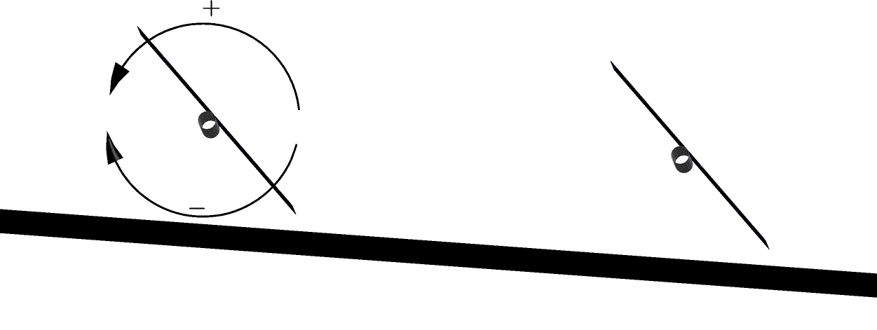
The ground slope itself is always positive, but the component of the slope perpendicular to the tracker axes can be positive or negative. The convention for the cross-axis slope angle follows the right-hand rule: align the right-hand thumb along the tracker axis in the direction of the axis azimuth and the fingers curl towards positive angles. So in this example, with the axis azimuth coming out of the page, an east-facing, downward slope is a negative rotation from horizontal:
Rotation curves
Now, let’s plot the simple case where the tracker axes are at right angles to the direction of the slope. In this case, the cross-axis tilt angle is the same as the slope of the terrain and the tracker axis itself is horizontal.
from pvlib import solarposition, tracking
import pandas as pd
import matplotlib.pyplot as plt

# PV system parameters
tz = 'US/Eastern'
lat, lon = 40, -80
gcr = 0.4

# calculate the solar position
times = pd.date_range('2019-01-01 06:00', '2019-01-01 18:00', closed='left',
                      freq='1min', tz=tz)
solpos = solarposition.get_solarposition(times, lat, lon)

# compare the backtracking angle at various terrain slopes
fig, ax = plt.subplots()
for cross_axis_tilt in [0, 5, 10]:
    tracker_data = tracking.singleaxis(
        apparent_zenith=solpos['apparent_zenith'],
        apparent_azimuth=solpos['azimuth'],
        axis_tilt=0,  # flat because the axis is perpendicular to the slope
        axis_azimuth=180,  # N-S axis, azimuth facing south
        max_angle=90,
        backtrack=True,
        gcr=gcr,
        cross_axis_tilt=cross_axis_tilt)

    # tracker rotation is undefined at night
    backtracking_position = tracker_data['tracker_theta'].fillna(0)
    label = 'cross-axis tilt: {}°'.format(cross_axis_tilt)
    backtracking_position.plot(label=label, ax=ax)

plt.legend()
plt.title('Backtracking Curves')
plt.show()
This plot shows how backtracking changes based on the slope between rows. For example, unlike the flat-terrain backtracking curve, the sloped-terrain curves do not approach zero at the end of the day. Because of the vertical offset between rows introduced by the sloped terrain, the trackers can be slightly tilted without shading each other.
Now let’s examine the general case where the terrain slope makes an inconvenient angle to the tracker axes. For example, consider an array with north-south axes on terrain that slopes down to the south-south-east. Assuming the axes are installed parallel to the ground, the northern ends of the axes will be higher than the southern ends. But because the slope isn’t purely parallel or perpendicular to the axes, the axis tilt and cross-axis tilt angles are not immediately obvious. We can use pvlib to calculate them for us:
# terrain slopes 10 degrees downward to the south-south-east. note: because
# slope_azimuth is defined in the direction of falling slope, slope_tilt is
# always positive.
slope_azimuth = 155
slope_tilt = 10
axis_azimuth = 180  # tracker axis is still N-S

# calculate the tracker axis tilt, assuming that the axis follows the terrain:
axis_tilt = tracking.calc_axis_tilt(slope_azimuth, slope_tilt, axis_azimuth)

# calculate the cross-axis tilt:
cross_axis_tilt = tracking.calc_cross_axis_tilt(slope_azimuth, slope_tilt,
                                                axis_azimuth, axis_tilt)

print('Axis tilt:', '{:0.01f}°'.format(axis_tilt))
print('Cross-axis tilt:', '{:0.01f}°'.format(cross_axis_tilt))
Out:
Axis tilt: 9.1°
Cross-axis tilt: -4.2°
And now we can pass use these values to generate the tracker curve as before:
tracker_data = tracking.singleaxis(
    apparent_zenith=solpos['apparent_zenith'],
    apparent_azimuth=solpos['azimuth'],
    axis_tilt=axis_tilt,  # no longer flat because the terrain imparts a tilt
    axis_azimuth=axis_azimuth,
    max_angle=90,
    backtrack=True,
    gcr=gcr,
    cross_axis_tilt=cross_axis_tilt)

backtracking_position = tracker_data['tracker_theta'].fillna(0)
backtracking_position.plot()

title_template = 'Axis tilt: {:0.01f}°   Cross-axis tilt: {:0.01f}°'
plt.title(title_template.format(axis_tilt, cross_axis_tilt))
plt.show()
Note that the backtracking curve is roughly mirrored compared with the earlier example – it is because the terrain is now sloped somewhat to the east instead of west.
Total running time of the script: ( 0 minutes 0.316 seconds)